Tech
How to use the FORMULATEXT function in Excel

The FORMULATEXT function is often dismissed because it merely transforms a formula into text. However, that raw text is exactly what makes it so valuable. So, stop thinking of it as a one-trick pony—it’s the perfect tool for auditing, input control, and logic validation.
The FORMULATEXT function has one argument:
=FORMULATEXT(ref)
where ref is a reference to a cell or, in modern versions of Excel, a range of cells.
If the ref argument is to another workbook, that workbook must be open. Otherwise, the formula will return the #N/A error. You’ll also see this error if the referenced cell doesn’t contain a formula.
Here are three ways you can use it in your spreadsheets today.
Debugging formulas
The simplest use of the FORMULATEXT function is straightforward formula auditing.
Suppose you’ve been sent a spreadsheet riddled with #DIV/0!, #VALUE!, #REF!, #SPILL!, and other errors. Selecting each cell one by one to review the formula in the formula bar is time-consuming. What’s more, spotting patterns in the errors is pretty much impossible.
Instead, you can use FORMULATEXT with IF and ISERROR in a single formula to only display the formulas of the cells where a problem is detected.
To do this, select the top-left cell where you want the formula audit to begin, and enter the following formula (replacing both cases of A2:D19 with the range you want to audit in your spreadsheet):
=IF(ISERROR(A2:D19),FORMULATEXT(A2:D19),"")
The result of this single formula spills across the entire audit area, returning only the formulas of cells containing errors.
This automatic spilling effect is available in Excel 2021 or later, Excel for Microsoft 365, Excel for the web, and the Excel tablet and mobile apps. In older versions, enter the formula as a legacy array formula by selecting all the cells in the audit area, typing the formula in the first selected cell, and pressing Ctrl+Shift+Enter to commit the formula to each cell.
This side-by-side view allows you to review the formulas instantly and diagnose the root causes of errors. As soon as you fix them, the formulas disappear from the audit area. What’s more, it lets you easily spot if the same faulty logic is applied to multiple cells.

These 5 little-known Excel features save me hours every week
My coworkers always wonder how I finish my Excel work so fast.
Documenting key formulas
You can use the FORMULATEXT to create a library of all the key formulas in your workbook. This has three main benefits:
- Improved understanding: It provides a central location where anyone can go to understand a workbook’s core logic.
- Streamlined handovers: If someone else is delegated to look after the workbook, the formula library serves as helpful documentation of how everything works.
- Formula safety net: You can periodically copy all the key formulas into another worksheet (paste values) or document for safekeeping. Date-stamp the pasted formulas to create a history of how a formula has evolved over time.
Creating a formula key is simple, involving just two columns on a dedicated worksheet: a formula label in column A and the formula text in column B.
Now, go through each worksheet, and each time you hit a cell containing an important formula—such as the final gross profit calculation on your Sales worksheet—type a formula label in column A, and in column B, type:
=FORMULATEXT(
Then, select the key cell, close the parentheses, and press Enter.
Finally, repeat the process for all the other key formulas in your workbook.
Format your key formula library as an Excel table. That way, each time you type a formula label on a new row in column A, the table will expand to capture the latest addition, housing your index within a single, nameable object.
Checking formula consistency
If you manage a large dataset, you’ll know that formula consistency down a column is one of your biggest quality control headaches.
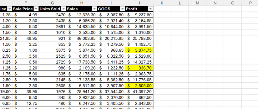
For example, if someone accidentally overwrites a formula with a hard-coded number or another formula, because the cell appears to have the correct information, the error goes undetected. In this spreadsheet, even though cells J8, J11, and J14 look legitimate at first glance, they don’t contain the same underlying mechanics as the other cells in column J.
When used alongside conditional formatting, the FORMULATEXT function helps you deal with this problem.
First, make sure the formula in the first cell of the column is correct, as this will be used as an absolute anchor cell against which you will verify the consistency of the rest of the column. Next, select the column you want to check (excluding the anchor) by selecting the second cell and pressing Ctrl+Shift+Down Arrow. Then, in the Home tab, click Conditional Formatting > New Rule.
Now, click “Use A Formula To Determine Which Cells To Format,” and enter the following formula (assuming you want to check column J):
=IF(NOT(ISFORMULA(J3)),TRUE,IF(NOT(ISFORMULA($J$2)),FALSE,FORMULATEXT(J3)<>FORMULATEXT($J$2)))
where:
- IF(NOT(ISFORMULA(J3)),TRUE checks if the current cell is a hard-coded value. If it is (TRUE), all other checks are bypassed, and the cell returns TRUE immediately.
- IF(NOT(ISFORMULA($J$2)),FALSE checks if the anchor cell is a hard-coded value. If it is, the process is stopped (FALSE).
- FORMULATEXT(J3)<>FORMULATEXT($J$2)) checks whether the current cell contains a formula that differs from the anchor cell (J2). If so, it returns TRUE.
Because the reference to cell J3 is relative, the conditional formatting rule adjusts for each row. On the other hand, the anchor cell is absolute (hence the dollar signs), so it consistently serves as the point of comparison.
Next, click “Format,” and choose a yellow cell fill to make the inconsistencies stand out.
Finally, click “OK” twice to close both dialog boxes and see the result.
If the anchor cell is a hard-coded value, no cells will be highlighted, so you run the risk of interpreting the column as error-free rather than the check having been aborted. This is why it’s crucial you double-check the anchor cell for accuracy.
As soon as you correct the formula in a highlighted cell, it will lose the formatting—and, before you know it, you’ll end up with an error-free, consistent spreadsheet.
Excel offers many ways to audit your spreadsheet. One of my favorites is the Go To Special tool, which lets you quickly select and edit all cells of a specific type—such as all cells containing formulas, constants, or conditional formatting. However, this built-in tool only tells you where the formulas are. By treating the formula as a text string, the FORMULATEXT function transforms from a simple viewer into a powerful quality control tool.

- OS
-
Windows, macOS, iPhone, iPad, Android
- Free trial
-
1 month
Microsoft 365 includes access to Office apps like Word, Excel, and PowerPoint on up to five devices, 1 TB of OneDrive storage, and more.


